A complete explanation from first principles
Reconstruction is a family of learning tasks
Reconstruction predicts a target from an incomplete or transformed input. An autoencoder may recover input from a compressed representation, a denoiser from a corrupted input, and masked image modeling from visible regions. Their targets and execution paths differ despite a shared missing-information idea.
Visible and hidden content have structure: edges continue, shapes repeat and objects co-occur. Learning those relationships may produce useful representations. Successful reconstruction alone does not establish comprehensive semantic understanding.
MAE separates a heavy encoder from a lighter decoder
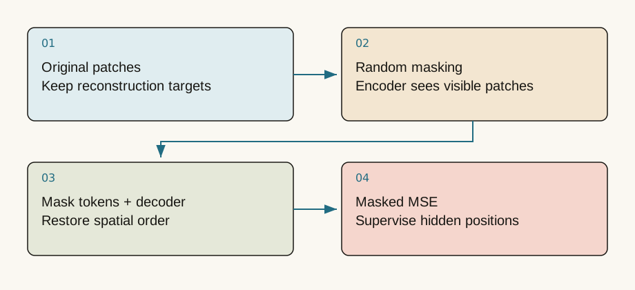
A key original MAE design sends only visible patches through the encoder. A lighter decoder receives their representations plus mask tokens, restores positional order and predicts pixels. For 196 patches and a 75% mask, the encoder processes 49 visible patches while the decoder returns to the full grid.
This differs from painting masked regions black while still running every position through the complete encoder. A mask token represents an unknown location rather than a black pixel patch. Incorrect restoration order can preserve output shape while scrambling the reconstructed image.
Specify which locations contribute to loss
For target patch y and prediction y_hat, MSE averages squared component differences. The usual MAE objective focuses on masked patches. Including large visible regions that are directly copied can dilute reported error and create a misleadingly favorable aggregate.
For target [0,1] and prediction [0.2,0.6], squared errors are [0.04,0.16], giving MSE 0.10. This measures numerical differences, not whether the output depicts the same cat. Normalized-pixel targets also require consistent handling of patch statistics when interpreting or displaying predictions.
Low MSE and perceptual sharpness are different
If the visible context permits several plausible hidden textures, a single squared-error predictor tends toward their conditional mean. Averaging possibilities can look blurry even when optimization succeeds. Conversely, a low pixel error can favor easy backgrounds without providing strong object representations.
Evaluate representations with separate probes, fine-tuning, retrieval or task-specific tests. Attractive reconstruction examples are not a substitute for those measurements.
Train an inspectable browser baseline
The notebook generates a smooth grayscale image, hides 75% of pixels, and fits z=a*x+b*y+c using visible pixels. Parameter updates and masked-region MSE are computed live. This is a linear reconstruction baseline, not a complete MAE architecture. It isolates what is observed, what is fitted and where quality is measured.
Replacing the target with a checkerboard exposes its limitation: a linear function cannot express alternating texture. Success on the first image depended on that image's smooth structure rather than general visual understanding.
The full PyTorch notebook uses actual pretrained MAE weights and shows the source, mask and reconstruction. A composite visualization may copy visible regions from the original, so inspect the masked regions separately. Record seed, mask ratio, preprocessing, target normalization and checkpoint. Hold the image fixed while changing the mask, then hold the mask fixed while changing the image. Separating those variables turns a gallery of outputs into an interpretable experiment.
Hide inputs to create supervision
Masked autoencoding removes patches and predicts missing content from visible regions. The original image supplies targets without manual category labels. MAE encodes only visible patches, then inserts mask tokens and positions in a decoder to restore sequence order. Downstream tasks commonly reuse the encoder, not the reconstruction decoder as a recognition head.
For 196 patches and 75% masking, 49 remain visible. CLS and implementation details may add another token. Shortening the encoder sequence does not reduce total model compute by exactly 75%, because decoding and projections remain.
Which positions contribute to loss?
A simplified masked MSE is , with squared error averaged within each patch and m=1 meaning hidden. This differs from the common attention-mask convention where one means valid. Supervising hidden patches avoids rewarding only direct copying.
import torch
pred = torch.zeros(1, 4, 3)
target = torch.ones_like(pred)
mask = torch.tensor([[1.,0.,1.,0.]])
per_patch = ((pred-target)**2).mean(-1)
loss = (per_patch*mask).sum()/mask.sum()
assert loss.item() == 1.0
Normalizing patch targets changes the loss and reconstruction display. Inspect settings such as norm_pix_loss; arbitrary logits are not automatically 0–255 pixels.
Attractive reconstruction is not stronger understanding
Pixel objectives reward texture and low-level detail; semantic tasks may require invariance to lighting or background. Latent-prediction approaches change the target space but must address issues such as representation collapse. Compare reconstruction error and transfer performance separately. A visually pleasing completion does not establish better retrieval or classification.
The on-page experiment uses synthetic grayscale patches and a constant predictor. It is untrained. The notebook loads actual facebook/vit-mae-base weights, fixes the random mask and displays the original, masked and reconstructed image together with model loss.
Check your understanding
Question: Does zero loss with zero mask ratio imply perfection?
Answer
No hidden positions are supervised and the denominator is zero. Training should reject the setting or define empty loss explicitly. The calculator's zero is only a display convention.Actual output from this run
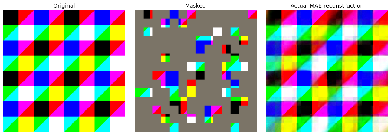
Actual vit-mae-base reconstruction of a synthetic color grid. This is neither a hand-filled image nor a natural-image quality benchmark.
Primary sources and further reading
Sources checked on 2026-09-10. Teaching examples are not production benchmarks; confirm APIs and model support against the linked version.
INTERACTIVE LAB · LIVE NUMERICAL COMPUTATION
Mask patches; measure loss only on hidden positions
An 8×8 synthetic grayscale grid. Adjust the mask and constant predictor to inspect masked MSE. This is not a trained MAE; the notebook runs real pretrained reconstruction.
With no masked patches there is no reconstruction supervision; zero is an empty-set convention, not perfect prediction.