Megatron-LM: what do TP, PP, DP and sequence sharding split?

Separate four partitioning choices

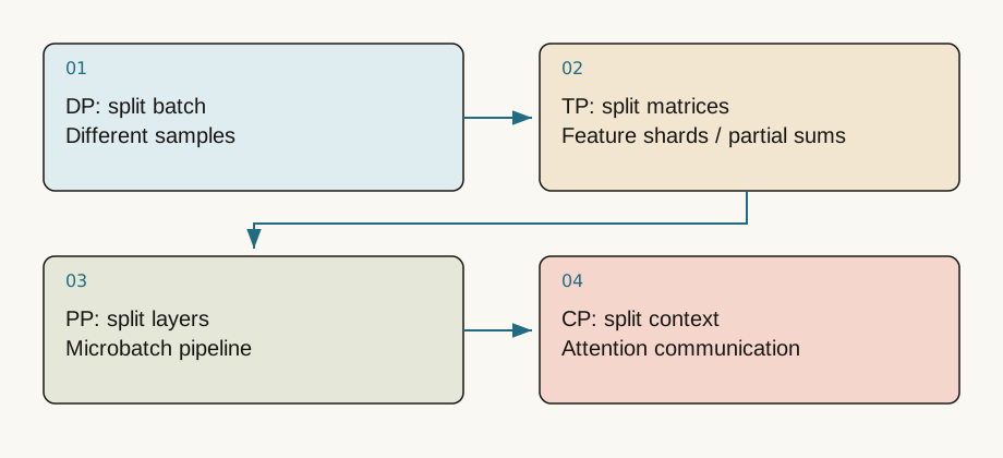
Data parallelism assigns different samples to replicas and synchronizes gradients. Tensor parallelism splits operations within a layer. Pipeline parallelism places layers on stages and moves microbatches through them. Context parallelism distributes long sequences and exchanges information needed by attention. Megatron's sequence parallelism commonly complements TP for selected activations and operations; it is not identical to full long-context attention partitioning.

Split a linear layer

Using row-vector notation, $Y=XW$ with X [B,T,D] and W [D,M]. Column parallelism splits W along output features M. A following row-parallel layer uses matching input-feature shards, computes partial sums and combines them through a collective. Proper composition can avoid gathering every intermediate activation.

import torch
x, w = torch.randn(3, 8), torch.randn(8, 12)
column_parts = [x @ p for p in w.chunk(2, dim=1)]
assert torch.allclose(torch.cat(column_parts, dim=1), x @ w)
row_parts = [a @ b for a,b in zip(x.chunk(2,1), w.chunk(2,0))]
assert torch.allclose(sum(row_parts), x @ w, atol=1e-6)

This single-process simulation verifies algebra, not distributed speed.

Put communication in the budget

An ideal ring all-reduce transfers approximately $2(P-1)S/P$ bytes per rank for an S-byte tensor. It omits startup latency and topology. Small tensors can be latency-bound; large ones depend more on effective bandwidth. Peak intra-node link speed cannot stand in for multi-node network behavior.

For a simplified flushed pipeline schedule, bubble fraction is approximately $(p-1)/(m+p-1)$, with p stages and m microbatches. Increasing m reduces this fraction but changes batching, activation memory and scheduling. Interleaving, 1F1B and recomputation need schedule-specific analysis.

Check your understanding

Question: Does increasing TP from two to eight necessarily reduce layer latency?

Answer

No. Smaller GEMMs can be less efficient and collective latency can dominate. First determine whether sharding is needed for memory, then measure strong scaling on the actual topology.

Primary sources and further reading

• Megatron Core features
• Megatron-LM
• Sequence parallelism

Sources checked on 2026-09-10. Teaching examples are not production benchmarks; confirm APIs and model support against the linked version.