Through ETEGRec, our central question was how an item becomes a token. Industrial recommendation presents a larger mountain:
billions of dynamic IDs
hundreds or thousands of heterogeneous features
user histories approaching 10⁵ actions
tens of billions of new actions per day
strict QPS and latency constraints
Putting a Transformer on a small dataset does not solve these problems. Actions Speak Louder than Words: Trillion-Parameter Sequential Transducers for Generative Recommendations does not begin by feeding product titles to an LLM. It asks:
What if user actions are a generative-modeling modality, ranking and retrieval become sequential transduction, and the architecture is redesigned for that data?
Its result, HSTU, marks this series' transition from academic prototypes to an industrial backbone.
The paper in 30 seconds
- The Semantic-ID branch's limitation: small catalogs, short histories, and beam-search experiments do not establish viability for billion-user systems with nonstationary vocabularies.
- HSTU's answer: merge heterogeneous features into a timeline and supervise many positions in one user-level pass; scale with pointwise aggregated attention, temporal bias, gating, Stochastic Length, ragged kernels, and M-FALCON.
- The evidence: HSTU-large improves NDCG@10 over SASRec by 65.8% on Amazon Books; HSTU is 5.3–15.2× faster than FlashAttention2 Transformers at length 8,192; an industrial GR reaches 1.5T parameters and reports +12.4% on a primary online ranking metric.
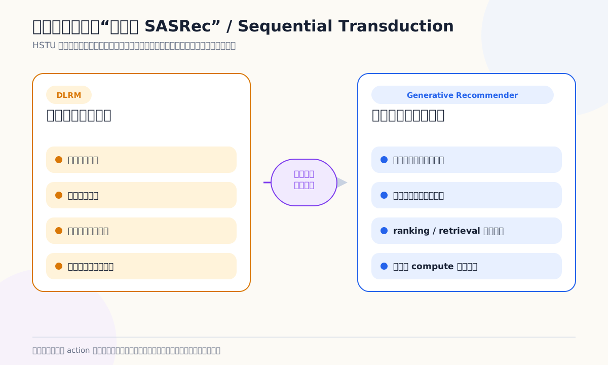
Figure 1. “Generative” here first describes data and training. It need not mean natural-language output or Semantic IDs.
The problem left by item tokenization
A traditional DLRM creates one example per (user, candidate):
user features + behavior statistics + candidate features
+ cross features → click/watch probability
This is controllable and battle-tested, but scaling has two bottlenecks:
- the same user history is encoded again for every candidate;
- quality often saturates before compute when larger cross networks and MLPs are added.
Academic sequential recommenders usually preserve only item IDs and discard creator, language, location, counter, ratio, and other production features. HSTU's first decision is therefore data arrangement, not a neural block.
Turning heterogeneous features into a timeline
Engaged items form the main categorical time series. Slowly changing sequences—followed creators, city, community, language—are compressed by keeping the first value of each consecutive segment and merged into the timeline.
Continuous numerical features are harder. Decayed counters and historical CTRs change at nearly every event, so fully sequentializing them is infeasible. The paper makes a strong assumption:
If the raw categorical events and target candidate are in the sequence, a sufficiently expressive target-aware model can relearn those aggregates, allowing many hand-engineered numerical features to be removed.
MTGR will challenge this assumption later. Here, it enables scaling by asking the model to summarize longer raw histories rather than storing every handcrafted summary.
Ranking and retrieval with eight items
Interleave content (\Phi_i) and response (a_i):
I01 tennis racket, click,
I03 climbing shoes, complete,
I05 badminton racket, skip,
I07 swim cap, save
Ranking: candidate in, action out
If the next token is candidate I06 goggles, predict:
[ P(a_{i+1}\mid \Phi_0,a_0,\ldots,\Phi_{i+1}). ]
The target participates in attention early, enabling target-aware interaction with the full history. The output can contain multitask logits for click, completion, and watch time.
Retrieval: history in, positive content out
At positive engagement positions, learn:
[ P(\Phi_{i+1}\mid u_i). ]
If an exposure was skipped, its target can be (\varnothing) rather than treating every shown item as desired content.
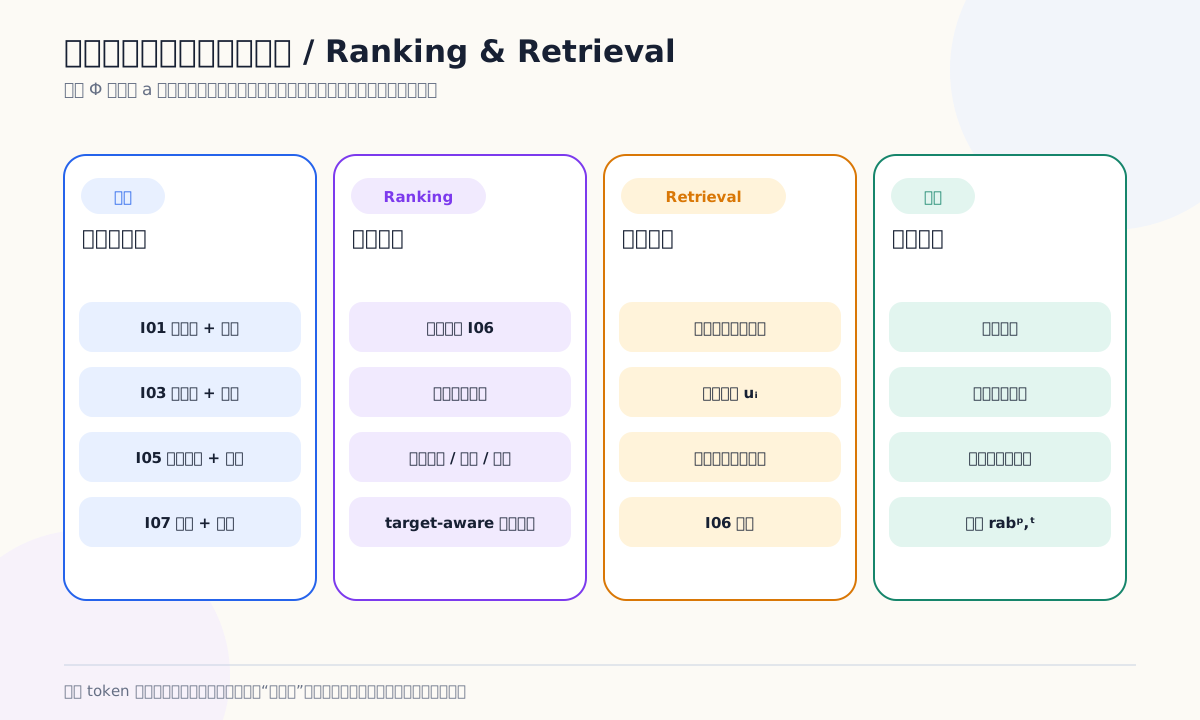
Figure 2. One token stream emits different supervision at different positions. The backbone is unified; the outputs are not forcibly identical.
Why user-level generative training saves a factor
Impression-level streaming repeatedly rebuilds every prefix. For user length (n_i), the paper writes cost as:
[ \sum_i n_i(n_i^2d+n_id^2). ]
With maximum length (N), that becomes approximately:
[ O(N^3d+N^2d^2). ]
Generative training supervises many positions in one full-sequence pass, amortizing encoder work across targets. Sampling a user at (s_u(n_i)\propto1/n_i) reduces cost to:
[ O(N^2d+Nd^2). ]
Attention remains quadratic. The saved factor comes from no longer recomputing the same prefix (N) times. A production system can emit one training example at the end of a request or session.
What an HSTU layer changes
An HSTU layer computes:
[ U,V,Q,K=\operatorname{Split}\big(\phi_1(f_1(X))\big), ]
[ A(X)V=\phi_2\big(QK^\top+\operatorname{rab}^{p,t}\big)V, ]
[ Y=f_2\Big(\operatorname{Norm}(AV)\odot U\Big). ]
(\phi_1,\phi_2) are SiLU; (\operatorname{rab}^{p,t}) encodes both relative position and elapsed time.
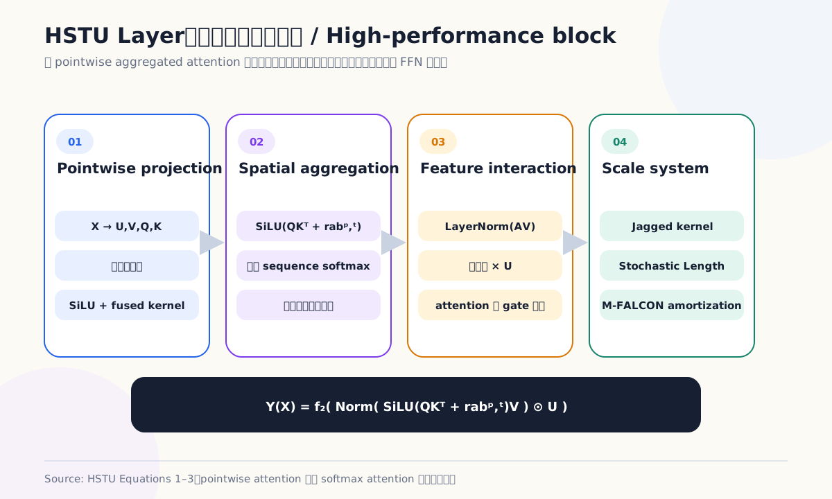
Figure 3. Attention aggregation and elementwise gating meet in one lightweight block with only two outer linear projections.
No sequence-wise softmax
Softmax normalizes each attention row to total mass one. If relevant history grows from two events to twenty, total mass remains one, making “how much supporting behavior exists” difficult to retain.
HSTU applies pointwise SiLU to (QK^\top), without normalizing across sequence positions, and then LayerNorms the pooled value. It can express both relevance and count. On synthetic streaming data, Transformer HR@10 is 0.0442, HSTU without time bias is 0.0893, and replacing pointwise activation with softmax yields 0.0617.
Gating instead of a separate FFN
(\operatorname{Norm}(AV)\odot U) directly mixes pooled history with a pointwise gate, related to SwiGLU and conditional computation. The paper estimates (14d) bfloat16 activation state per HSTU layer versus (33d) for a Transformer, allowing a substantially deeper network under the same memory budget.
Three more scaling components
Ragged kernels
History lengths are highly skewed. Padding every user to the maximum wastes most compute. HSTU uses fully ragged grouped GEMMs and fused kernels.
Stochastic Length
Long histories repeat at multiple time scales. Training usually samples a shorter subsequence from very long users but occasionally retains the full history. With (\alpha=1.6), length 4,096 becomes 776 most of the time. The paper reports no more than 0.002 degradation in major normalized-entropy tasks at 64%–84% sparsity.
M-FALCON
Ranking still processes many candidates. M-FALCON microbatches candidates and caches candidate-independent history work. The paper serves a 285× more computationally complex GR while obtaining 1.50×/2.99× the DLRM QPS when scoring 1,024/16,384 candidates.
What the experiments establish
Full-ranking public results are:
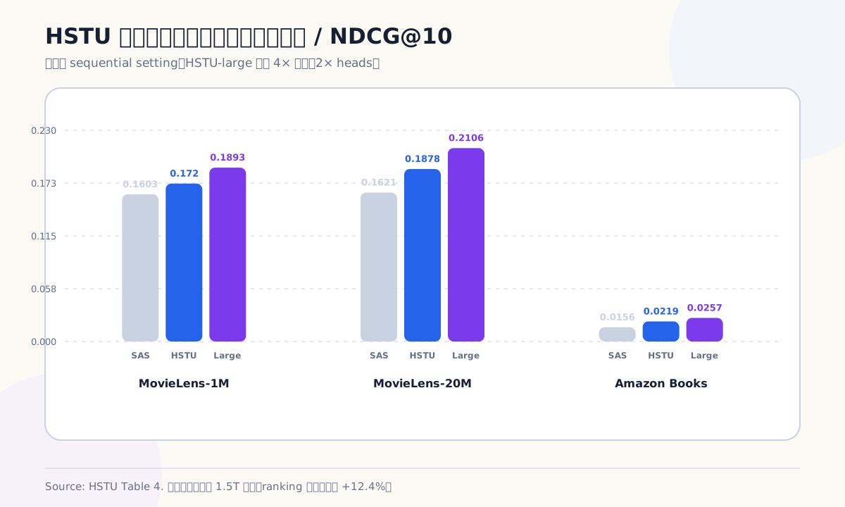
Figure 4. Relative gains are largest on sparse Amazon Books, and scaling HSTU improves all three datasets.
| Dataset | SASRec | HSTU | HSTU-large |
|---|---|---|---|
| MovieLens-1M | 0.1603 | 0.1720 | 0.1893 |
| MovieLens-20M | 0.1621 | 0.1878 | 0.2106 |
| Amazon Books | 0.0156 | 0.0219 | 0.0257 |
In one-pass industrial streaming, full HSTU has retrieval log perplexity 3.978 versus Transformer++ at 4.015. Its primary ranking-task normalized entropy is 0.4937 versus 0.4945, lower being better.
The scaling observation is more consequential:
- retrieval HR@100, HR@500, and ranking NE follow log/power-law fits over three orders of compute;
- GR scales to 1.5T parameters, whereas DLRM quality saturates around 200B parameters;
- the largest configuration uses length 8,192, embedding width 1,024, and 24 HSTU layers;
- the production ranking model reports +12.4% on its primary online task and +4.4% on a secondary task.
The 1.5T count includes high-cardinality embedding parameters. It is not computationally equivalent to a 1.5T dense LLM. The comparison concerns recommendation's own capacity–compute–quality relationship.
Where HSTU breaks
Core industrial evidence is not reproducible
The 1.5T model, private data, online metrics, and serving kernels cannot be reproduced through public benchmarks. Open code validates the block, not the complete claim.
A scaling law is an empirical fit
The curves cover one platform's tasks and configurations. Data quality, feedback labels, sequence length, and embedding capacity change together. They do not imply that adding compute improves every recommender.
Pointwise attention trades away automatic normalization
Softmax bounds total mass and suppresses many weak events. Pointwise aggregation relies on LayerNorm, data processing, and kernels for stability; not every long-history event is useful.
Removing numerical features is a strong assumption
A sequence can theoretically relearn CTR, exposures, and crosses. Under finite context, capacity, and drift, explicit statistics may remain more efficient. MTGR provides direct production evidence for that objection.
Unified representation is not yet one list objective
Ranking predicts actions and retrieval predicts content. They share a sequential-transduction backbone, but recall, ranking, policy, and list constraints are not one generated session.
Why OneRec comes next
HSTU establishes an industrial backbone that scales and puts many tasks on one behavior timeline. A deployed system may still retain retrieval, pre-ranking, and ranking:
unified backbone ≠ unified final decision
OneRec, in the next chapter, takes another step: one encoder–decoder generates a 5–10-video session, Sparse MoE expands capacity, and a reward model plus DPO aligns the final list to watch and interaction preferences.
Critical takeaway: HSTU is not one attention equation. Scaling appears only after the problem is rewritten at four layers: aggregate data by user, formulate tasks as transduction, compute over real ragged lengths, and amortize candidate cost through caching. A trillion parameters matters only when all four are true.