Recommender Systems Began as Scoring Machines | Generative Recommendation 01: BPR

Lin clicked a pair of climbing shoes and did not click a pair of swimming goggles.

Does that mean she dislikes the goggles?

Not necessarily. She may never have seen them. She may be shopping only for climbing equipment today. She may already own a pair. This is the normal state of recommendation data: implicit feedback records clicks, dwell time, carts, and purchases, surrounded by a much larger volume of unexplained silence.

If we label every interaction as 1 and every missing interaction as 0, a classifier is forced to treat all silence as explicit rejection. BPR: Bayesian Personalized Ranking from Implicit Feedback asks a narrower question:

We may not know the rating Lin would assign to every item. If she interacted with item $i$ but not item $j$, can we at least learn to rank $i$ above $j$?

This is the first foundation of the series. Whether later models use a GRU, a Transformer, an LLM, or Semantic IDs, they still need some answer to the same question: what training signal puts the right item above the wrong one?

Understand the paper in 30 seconds

1. The earlier limitation: implicit feedback says what happened, but supplies no reliable negative ratings; fitting pointwise values is also misaligned with the final Top-K ranking task.
2. BPR’s answer: construct a triple $(u,i,j)$ from an observed item $i$ and an unobserved item $j$, then maximize $\sigma (s(u,i)-s(u,j))$, the modeled probability that user $u$ prefers $i$.
3. The decisive evidence: the paper attaches the same BPR criterion to matrix factorization and adaptive kNN, improving personalized ranking in both cases. Its primary contribution is an objective and learning procedure, not a new neural architecture.

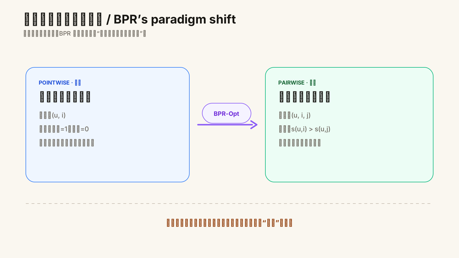
Figure 1. BPR’s important move is not a larger scorer. It replaces absolute-value fitting with relative ordering for the same user.

What problem did the previous paradigm leave behind?

Explicit feedback is easy to describe. If Lin gives a tennis racket five stars and a yoga mat two, a model can regress those numbers.

Most recommendation logs do not contain ratings. Let $\mathcal{U}$ be the users, $\mathcal{I}$ the items, and

$$S\subseteq \mathcal{U}\times \mathcal{I}$$

the observed interactions. The statement $(u,i)\in S$ only says that user $u$ performed some action on item $i$. It does not reveal:

• whether a click meant genuine preference;
• whether a missing click meant dislike or no exposure;
• which of two observed items the user prefers;
• or how two unobserved items should be ordered.

A pointwise solution can call observed pairs positive and every other pair negative. For a million-item catalog, however, every positive is surrounded by nearly a million ambiguous “negatives.”

BPR accepts the ambiguity and limits the inference:

• if $i$ is observed and $j$ is unobserved, assume $i\succ_u j$;
• infer no ordering between two observed items;
• infer no ordering between two unobserved items.

It does not prove that “unclicked means disliked.” It says:

Given the weak evidence available in this log, first place an item with observed behavior above one covered only by silence.

Understand the training data with eight items

We will reuse Lin and the same eight sports items throughout the series. Suppose she clicked I03 climbing shoes and has no interaction with I06 goggles.

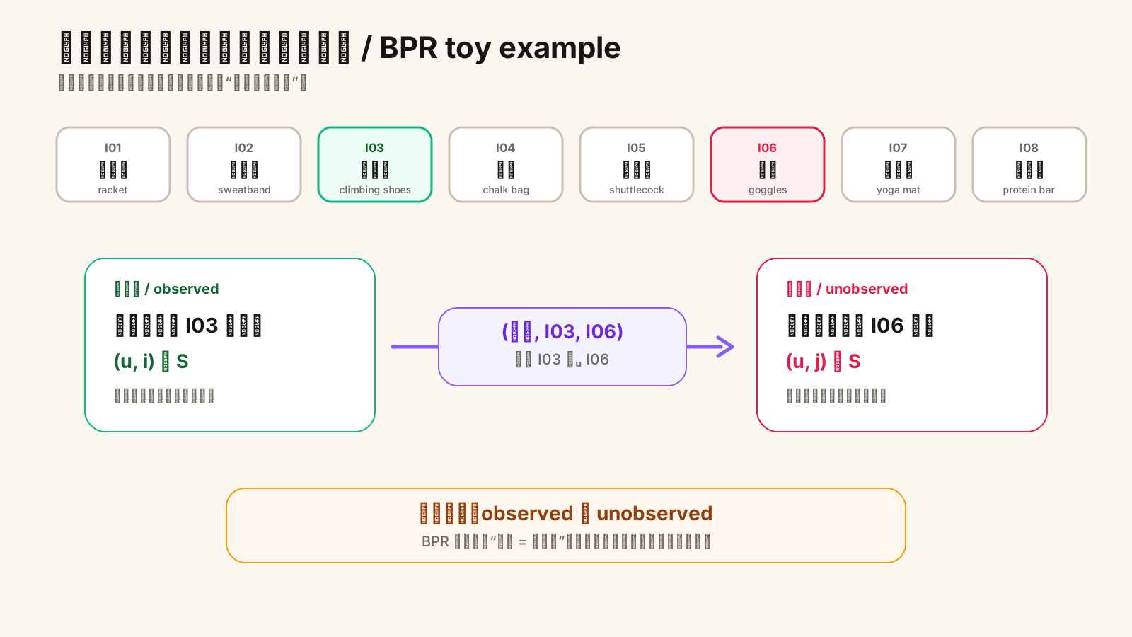
Figure 2. BPR constructs $(u,i,j)$ from one observed and one unobserved item. The preference is a training assumption, not a statement the user made.

For user $u$, define the observed set as

$${\mathcal{I}}_u^{+}=\{i\in \mathcal{I}\mid (u,i)\in S\}.$$

The training relation is

$$D_S=\{(u,i,j)\mid i\in {\mathcal{I}}_u^{+},j\in \mathcal{I}\setminus {\mathcal{I}}_u^{+}\}.$$

The triple (Lin, I03, I06) does not mean “the shoes have label 1 and the goggles label 0.” It represents the binary ordering statement

$$I03{\succ }_{\text{Lin}}I06.$$

That distinction changes the gradient:

• a pointwise loss separately moves $s(u,I03)$ toward 1 and $s(u,I06)$ toward 0;
• a pairwise loss only needs the margin $\Delta =s(u,I03)-s(u,I06)$ to become positive and sufficiently large.

Scores of 101 and 100 look strange as probabilities but have the correct order. Scores of 0.8 and 0.9 look individually plausible yet rank the items incorrectly. BPR optimizes the latter distinction.

What happens from model input to output?

BPR is not one fixed scorer. It is an optimization framework that can sit on top of different model classes. The paper demonstrates matrix factorization and adaptive kNN. The canonical combination is BPR-MF.

Assign $d$-dimensional embeddings to users and items:

$${\mathbf{w}}_u\in {\mathbb{R}}^d,{\mathbf{h}}_i,{\mathbf{h}}_j\in {\mathbb{R}}^d.$$

The user–item score is

$${\hat{x}}_{ui}={\mathbf{w}}_u^{\top }{\mathbf{h}}_i,$$

and the pairwise margin is

$${\hat{x}}_{uij}={\hat{x}}_{ui}-{\hat{x}}_{uj}={\mathbf{w}}_u^{\top }({\mathbf{h}}_i-{\mathbf{h}}_j).$$

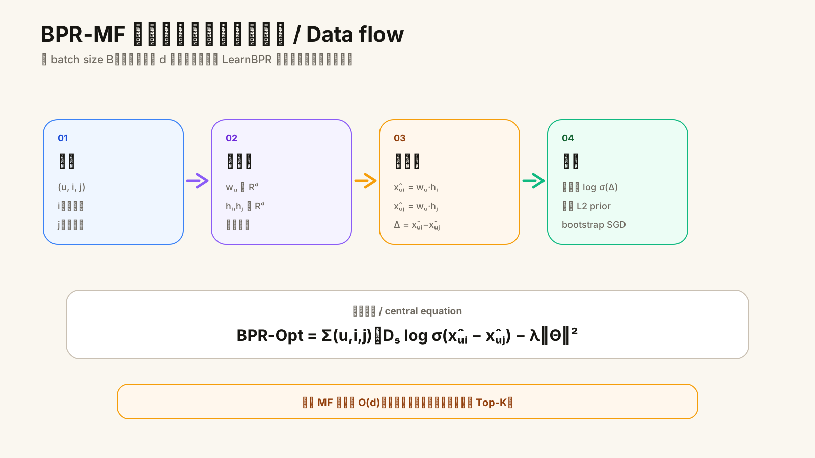
Figure 3. One update reads one user embedding and two item embeddings. Training enlarges their score difference; inference still scores candidate items.

For a mini-batch of $B$ triples, a modern implementation often contains:

Tensor	Shape	Meaning
user_ids	$[B]$	user indices
pos_item_ids	$[B]$	observed items
neg_item_ids	$[B]$	sampled unobserved items
user_emb	$[B,d]$	user vectors
pos_emb, neg_emb	$[B,d]$	positive and negative item vectors
margin	$[B]$	${\hat{x}}_{ui}-{\hat{x}}_{uj}$

One MF triple update costs roughly $O(d)$, so training does not have to materialize the enormous set $D_S$.

BPR is nevertheless still a scoring machine. At serving time it evaluates ${\hat{x}}_{ui}$ for candidates and selects Top-K. It does not generate an item token, and the second result does not condition on the first. It begins this history because it establishes the prototype for later ranking supervision.

Unpack the central equation

BPR models the probability of the pairwise preference as

$$p(i{\succ }_{u}j\mid \Theta )=\sigma ({\hat{x}}_{uij})=\frac{1}{1+\exp (-{\hat{x}}_{uij})}.$$

With a zero-mean Gaussian prior over parameters $\Theta$, the maximum-posterior objective becomes

$$\mathrm{BPR}\text{-}\mathrm{Opt}=\sum _{(u,i,j)\in D_S}\log \sigma ({\hat{x}}_{uij})-\lambda \Vert \Theta {\Vert }_2^2.$$

Each term has a concrete job:

• ${\hat{x}}_{uij}$ is the positive–negative score margin;
• $\sigma ({\hat{x}}_{uij})$ maps it to a probability in $(0,1)$;
• $\log \sigma (\cdot )$ strongly penalizes a reversed pair but saturates once the pair is clearly ordered;
• $\lambda \Vert \Theta {\Vert }_2^2$ comes from the parameter prior and discourages solving the task merely by inflating embedding norms.

Written as a loss to minimize:

$${\mathcal{L}}_{\mathrm{BPR}}=-\log \sigma ({\hat{x}}_{ui}-{\hat{x}}_{uj})+\lambda \Vert \Theta {\Vert }_2^2.$$

For intuition:

• if the shoes score 1.2 and the goggles 0.2, $\Delta =1$, giving probability about 0.731;
• if their order is reversed, $\Delta =-1$, giving about 0.269 and a strong corrective gradient;
• if $\Delta =6$, the probability is already near 1, so enlarging the margin has little additional benefit.

This also explains the connection to AUC. AUC counts how often a positive item outranks a negative one. BPR replaces the non-differentiable pairwise indicator with the smooth $\log \sigma (\Delta )$.

Training versus inference

The full $D_S$ has order $O(|S||\mathcal{I}|)$ triples and cannot be enumerated. The paper proposes LearnBPR: repeatedly sample a user, an observed item, and an unobserved item, then perform an immediate stochastic update.

initialize user and item embeddings
repeat:
    sample user u
    sample observed item i from I_u+
    sample unobserved item j from I \ I_u+

    delta = score(u, i) - score(u, j)
    loss  = -log sigmoid(delta) + regularization
    update only w_u, h_i, h_j
until validation ranking stops improving

Random triples are more than an implementation convenience. An item-wise or user-wise traversal repeatedly strikes the same parameters, and popular positives create many closely related comparisons. Bootstrap sampling breaks up that skew and converges more effectively.

Inference is a different computation:

user_vector = W[u]
for candidate item i:
    score[i] = dot(user_vector, H[i])
return top_k(score)

Brute-force full-catalog scoring costs roughly $O(|\mathcal{I}|d)$. Production systems therefore narrow the set with retrieval, an approximate vector index, or cached candidates. BPR teaches a ranking; it does not solve million-item retrieval.

What do the experiments actually prove?

The original paper performs two useful controls:

1. keep matrix factorization as the model while comparing BPR with other learning criteria;
2. attach BPR to adaptive kNN to test whether the benefit belongs only to MF.

Across several implicit-feedback datasets, the authors evaluate personalized ranking with AUC and report that BPR-MF and BPR-kNN outperform their corresponding baselines. The durable conclusion is not one isolated number:

Holding much of the representation machinery constant, replacing value reconstruction with direct pairwise ranking can materially improve the final ordering.

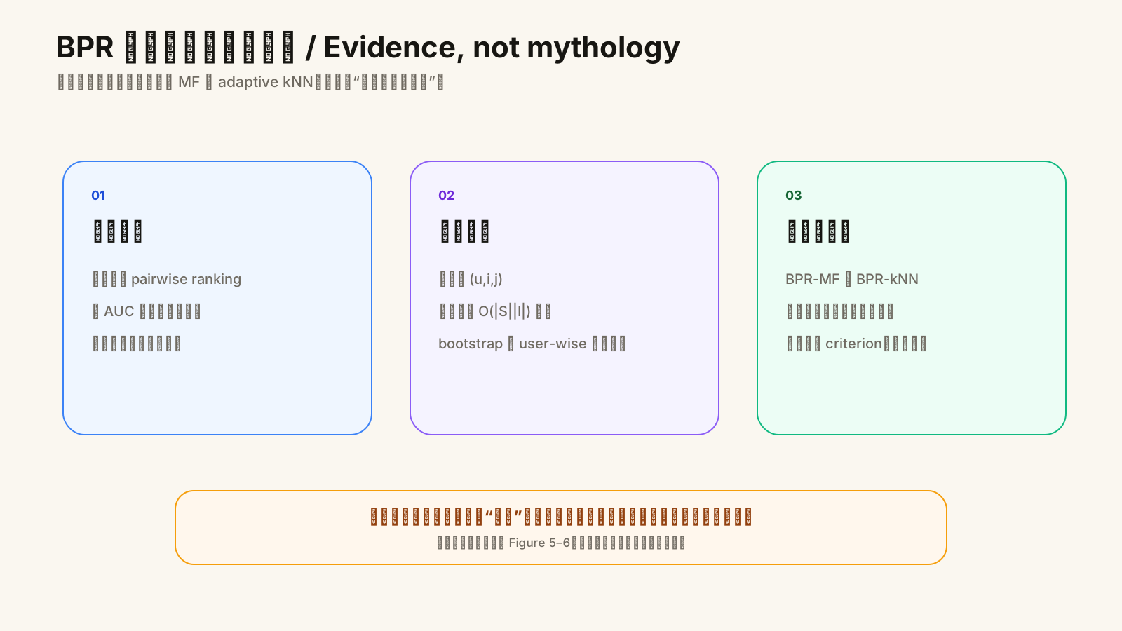
Figure 4. This redraw preserves the evidence structure of Figures 5–6 in the paper without inventing pseudo-precise values from plotted curves.

Three qualifications matter today:

• offline AUC is not online click-through rate, conversion, or long-term satisfaction;
• logged interactions inherit the exposure policy of the previous system;
• the results support BPR for these models and settings, not the universal superiority of pairwise objectives over stronger listwise or counterfactual methods.

Where does it fail?

1. No exposure and dislike become indistinguishable

BPR assumes $i{\succ }_{u}j$ whenever $i\in {\mathcal{I}}_u^{+}$ and $j\notin {\mathcal{I}}_u^{+}$. If I06 goggles was never shown, treating it as a negative teaches the blind spots of the old recommender.

This is exposure bias: a log records behavior after an existing policy selected what to display. It is not an unbiased map of preference over the entire catalog.

2. Negative sampling defines the learned boundary

Uniform sampling produces many trivially irrelevant negatives. Popularity sampling creates harder comparisons but may over-suppress popular items. Category-level hard negatives provide more information while increasing false negatives—two items may both be desirable.

The loss occupies one line; the sampling distribution can determine much of the model’s behavior.

3. One user has one static vector

BPR-MF compresses Lin into ${\mathbf{w}}_u$. If she liked tennis for a year but started climbing today, event order disappears into one coordinate. The model estimates “what kind of person she is,” not “what she is doing now.”

4. Independent scores do not naturally model a slate

Climbing shoes and a chalk bag may each score highly, but placing the shoes first does not directly change the value of the second slot. Diversity, complementarity, and duplication remain tasks for a downstream reranker.

5. Correct historical ranking is not a causal effect

BPR imitates ordering in logged behavior. It does not estimate whether showing an item causes greater satisfaction. Position, popularity, price, inventory, and the old policy all affect the data.

Why does the next paper need to exist?

BPR teaches the first necessary skill:

For one user, an observed item should score above a sampled unobserved item.

But the user remains a stationary point.

If Lin looks at a tennis racket and then climbing shoes, BPR-MF sees essentially the same interaction set as it would in the reverse order. The intent may be different: the former resembles broad sports browsing, while the latter may indicate preparation for tonight’s bouldering session.

The next paper therefore rewrites “who is the user?” as “how is this session unfolding?”

Next: GRU4Rec—a user is not a point, but a story in motion.

Original paper

• Steffen Rendle, Christoph Freudenthaler, Zeno Gantner, Lars Schmidt-Thieme. BPR: Bayesian Personalized Ranking from Implicit Feedback. UAI 2009; arXiv version 2012.

Return to the complete roadmap →