History Is Long, but Only a Few Steps May Matter | Generative Recommendation 03: SASRec

Lin has fifty recent actions. She bought a tennis racket, inspected badminton shoes, opened a pair of goggles, and purchased climbing shoes a month ago.

Now she is viewing a chalk bag.

Which event matters?

• the most recent click is usually useful;
• the climbing-shoe purchase a month ago may be more closely related;
• the tennis and swimming behavior in between may be noise.

GRU4Rec, the previous paper, recurrently compresses all fifty actions into one hidden state. In theory it can remember an old purchase. In practice, that information must survive dozens of state updates before reaching the present.

Self-Attentive Sequential Recommendation, or SASRec, takes a different route:

Do not force all history through one vector first. Let the current prediction compare itself directly with every past step and decide what matters.

The 2018 paper brings Transformer self-attention into sequential recommendation and pushes an Item ID another step toward being a token.

Understand the paper in 30 seconds

1. The limitation left by GRU4Rec: recurrent states are difficult to parallelize, early events have a long path to the current output, and all history is compressed into one vector.
2. SASRec’s answer: add position embeddings to Item IDs and use causal self-attention so position $t$ can inspect only $1,\dots ,t$, assigning different relevance to different actions.
3. The decisive evidence: on Amazon Beauty/Games, Steam, and MovieLens-1M, SASRec beats simple models on sparse data and RNN/CNN models on dense data. The paper reports average gains of 6.9% in Hit Rate and 9.6% in NDCG over the strongest baselines.

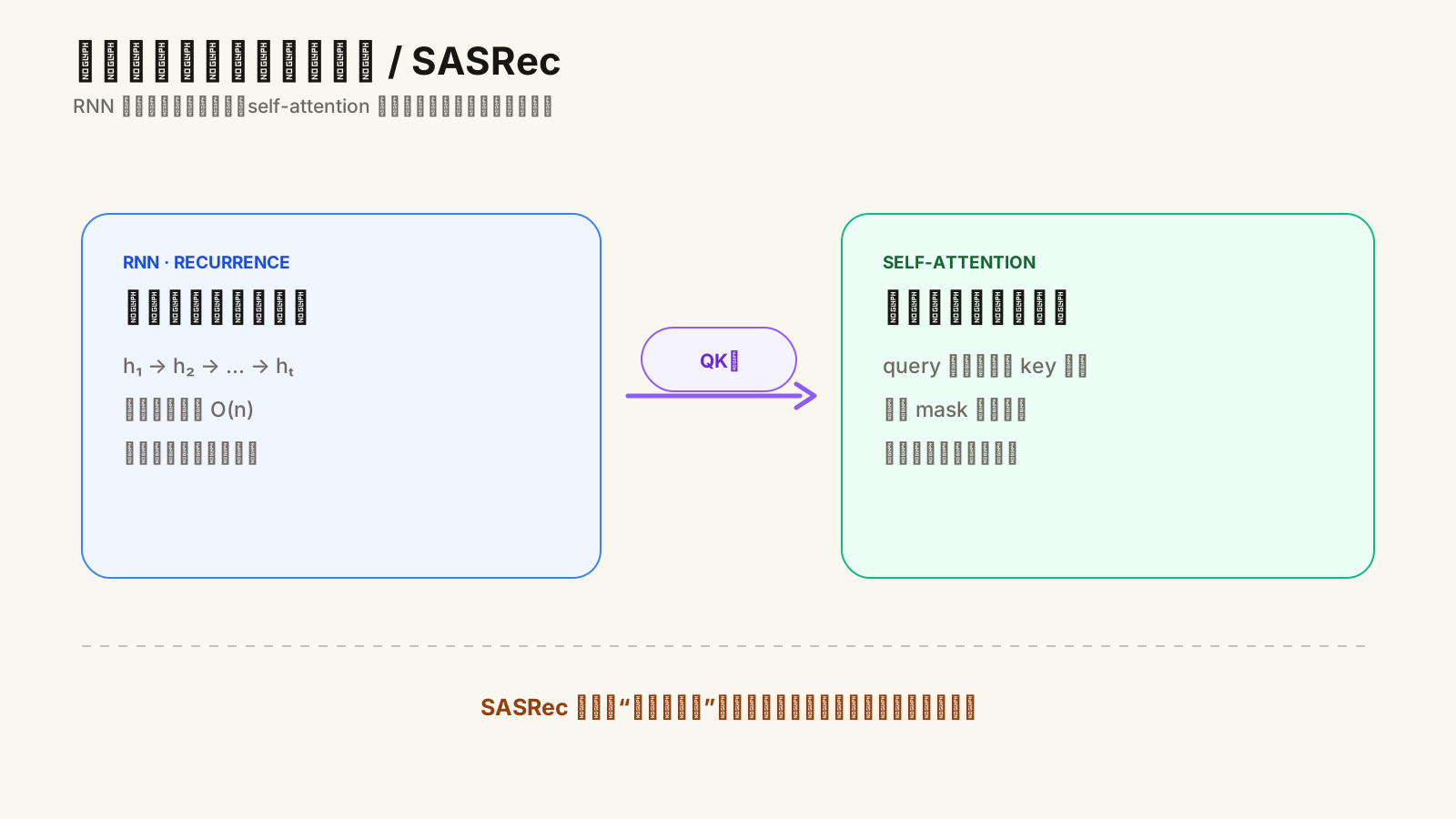
Figure 1. RNN information travels step by step. Self-attention gives the current position a one-hop path to every visible historical position.

What problem did the previous paper leave behind?

A GRU update is

$${\mathbf{h}}_t=f({\mathbf{x}}_t,{\mathbf{h}}_{t-1}).$$

This creates three structural constraints:

1. Information bottleneck: ${\mathbf{h}}_t$ must retain everything that any future request may need.
2. Maximum path $O(n)$: information from the first event crosses $n-1$ transitions before affecting event $n$.
3. Temporal dependency: step $t$ in one sequence waits for step $t-1$.

At the other extreme, a first-order Markov chain reads only the latest action. Its path is short and its parameterization compact, which can make it more robust than a large neural model on extremely sparse data.

SASRec aims to connect the two:

• retain the capacity to use long history like an RNN;
• focus on a few relevant actions like a Markov model;
• and calculate all training positions in parallel.

Use one history to understand attention

Suppose the visible history is

I01 racket → I03 climbing shoes → I05 shuttlecock

and the target is I06 goggles. SASRec neither hard-codes “use only the last item” nor averages all three equally. The current position creates a query; each historical position contributes a key and a value:

• the query may match I01 weakly;
• I03 may indicate a broader shift in sports interest;
• the recent I05 may receive an intermediate weight.

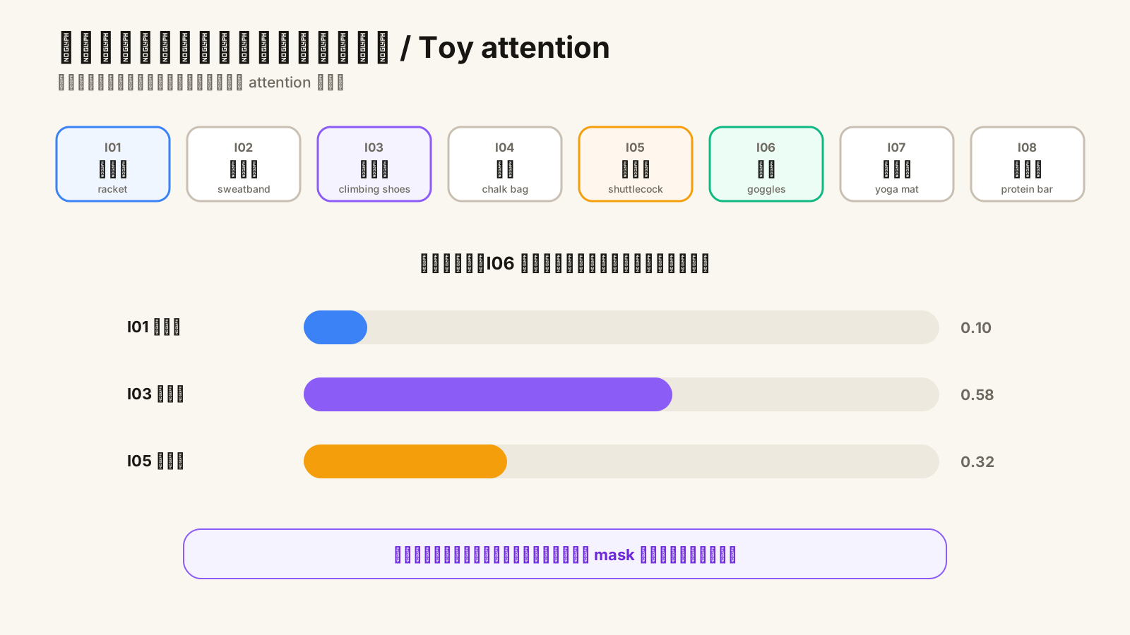
Figure 2. The values illustrate the mechanism; they are not measured attention weights for a user in the paper. Real attention is learned and changes across layers.

One restriction is essential. When predicting position $t+1$, the model must not see items after $t+1$. That would leak the answer during training. SASRec applies a causal mask, setting all future attention logits to negative infinity.

It is the same left-to-right rule used by decoder-only language models.

What happens from model input to output?

Let a user sequence be

$$S^u=(S_1^u,S_2^u,\dots ,S_{|S^u|}^u),$$

with maximum length $n$ and embedding width $d$.

1. Truncation, padding, and position

Keep the most recent $n$ actions and left-pad shorter sequences. Look up each item and add a learned positional vector:

$${\mathbf{E}}_t={\mathbf{M}}_{S_t^u}+{\mathbf{P}}_t,\mathbf{E}\in {\mathbb{R}}^{n\times d}.$$

An Item ID contains no order. Without ${\mathbf{P}}_t$, tennis → climbing and climbing → tennis are just two vectors in a set.

2. Causal self-attention

Linear projections produce

$$Q=\mathbf{E}{W}^Q,K=\mathbf{E}{W}^K,V=\mathbf{E}{W}^V.$$

The attention matrix is $n\times n$. Row $t$ specifies how the current position combines its visible history.

3. Residual paths, normalization, and position-wise FFN

Attention is followed by dropout, a residual connection, and layer normalization, then by a two-layer feed-forward network applied independently to every position. The default paper model stacks two self-attention blocks.

4. Score the next item

Representation ${\mathbf{h}}_t$ is dotted with candidate item embeddings:

$$r_{i,t}={\mathbf{h}}_t^{\top }{\mathbf{M}}_i.$$

Every position treats the real next item as positive and samples an unobserved item as negative, training with binary cross-entropy.

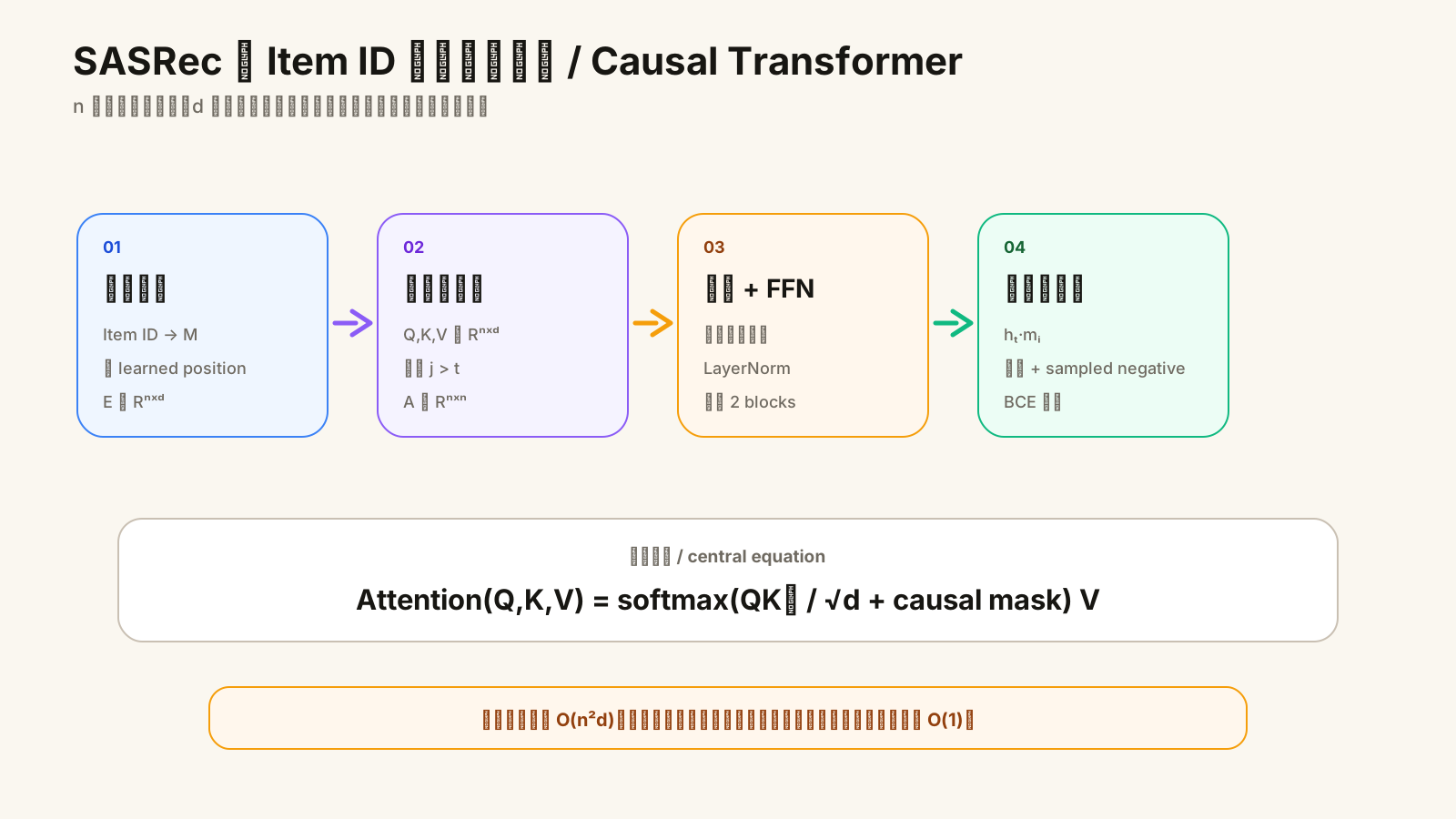
Figure 3. Each position reads only its left context. The output remains candidate-item scores, and item embeddings are shared between the input and prediction layers.

The key tensor shapes are:

Tensor	Shape	Meaning
item_ids	$[B,n]$	padded behavior sequences
embeddings	$[B,n,d]$	item plus position
attention_logits	$[B,n,n]$	relevance from every position to history
hidden	$[B,n,d]$	contextual state at every time step
positive_scores	$[B,n]$	true next-item scores
negative_scores	$[B,n]$	sampled negative scores

Unpack the central equation

The core operation is scaled dot-product attention:

$$\mathrm{Attention}(Q,K,V)=\mathrm{softmax}\left(\frac{Q{K}^{\top }}{\sqrt{d}}+M_{\text{causal}}\right)V.$$

Term by term:

• $Q{K}^{\top }$ measures the match between each current position and every historical position;
• $\sqrt{d}$ controls the variance of large-dimensional dot products and prevents premature softmax saturation;
• $M_{\text{causal}}$ is $-\infty$ for future positions and zero for visible ones;
• softmax turns each row into normalized weights over history;
• multiplying by $V$ aggregates historical information with those weights.

The difference from a GRU is deeper than “weighted averaging.”

Information from the first event reaches the final recurrent state through the full chain. Self-attention creates a direct edge. The paper summarizes the maximum path as:

• RNN: $O(n)$;
• self-attention: $O(1)$.

The price is an $n\times n$ matrix and approximately

$$O(n^{2}d+n{d}^2)$$

computation. This is manageable for $n=50$ or $200$ in the paper, but not for tens of thousands of industrial events without sparse attention, hierarchy, retrieval, or compression.

Training versus inference

Training shifts every sequence by one:

input : [PAD, I01, I03, I05]
target: [I01, I03, I05, I06]

Every non-padding position contributes a next-item objective:

for user sequence:
    keep the most recent n items and left-pad
    hidden = SASRec(item_embedding + position_embedding,
                    causal_mask=True)

    for every valid position t:
        positive = the real item at t + 1
        negative = sample one item not in the user sequence
        optimize BCE(score(hidden[t], positive),
                     score(hidden[t], negative))

Inference:

1. keep the most recent $n$ actions;
2. calculate all representations in parallel;
3. read the final non-padding state $\mathbf h_t$;
4. dot it with candidate item embeddings;
5. remove interacted or unavailable items and take Top-K.

Training is parallel over sequence positions, but full-catalog output may still cost $O(|\mathcal{I}|d)$. An external retriever or approximate nearest-neighbor index is needed when exhaustive scoring is too expensive.

What do the experiments actually prove?

The paper deliberately chooses datasets with very different sparsity:

Dataset	Users	Items	Actions/user
Amazon Beauty	52,024	57,289	7.6
Amazon Games	31,013	23,715	9.3
Steam	334,730	13,047	11.0
MovieLens-1M	6,040	3,416	163.5

This tests the central claim: compact Markov methods tend to be robust in sparse settings; expressive RNN/CNN models tend to become competitive in dense ones; can SASRec adapt across both?

Figure 4. Purple is SASRec; gray is the strongest neural baseline for each dataset. Values come from Table III of the paper.

The paper reports average gains over the strongest baseline of:

• 6.9% Hit Rate;
• 9.6% NDCG.

Examples:

• Beauty NDCG@10 increases from 0.2556 for the strongest neural baseline to 0.3219;
• Steam rises from 0.5595 to 0.6306;
• MovieLens-1M rises from 0.5538 to 0.5905.

The ablations are equally informative:

• removing positional embeddings slightly helps the sparsest Beauty data but hurts denser datasets, so the value of order depends on the data;
• unsharing input and output item embeddings hurts all four datasets substantially;
• removing residual connections, dropout, or every attention block usually produces a severe drop;
• at the paper’s relatively small $d$, the default single-head attention is not worse than the multi-head variant.

The authors also report about 1.7 seconds of model updates per epoch on one GTX 1080 Ti, faster than the compared Caser and GRU4Rec+ configurations. The hardware number is obsolete, but it supports the engineering argument that sequence positions can be parallelized.

Where does it fail?

1. Training remains left-to-right

The causal mask prevents leakage, which is necessary, but it also stops position $t$ from using right context. The complete training history is available, yet only one direction is used for each representation.

2. Quadratic attention cannot grow forever

$n=200$ gives forty thousand pairwise positions. $n=10,000$ gives one hundred million. SASRec demonstrates that attention works for recommendation; it does not solve very long industrial histories.

3. Every Item ID remains a private token

Embeddings for I03 and I04 can learn co-occurrence, but the IDs themselves carry no textual semantics. A new “climbing chalk bag” cannot be understood from its description without interaction or added content features.

4. Negative sampling and sampled evaluation change the task

Training uses one negative per position. Evaluation ranks the real next item against one hundred sampled negatives. That is easier than full-catalog retrieval and makes Hit@10 values from different papers unsafe to compare directly.

5. Attention is not a causal explanation

A high weight means the current computation relies more on a value. It does not prove that the historical event caused the recommendation, nor that the weight is a faithful human explanation.

6. The objective is still one next item

Every position predicts an item independently. Diversity, cross-item dependence, inventory, and long-term objectives remain outside the model. SASRec is a powerful sequential scorer, not a complete generative system.

Why does the next paper need to exist?

SASRec has made a shopping history look much more like a sentence:

• Item IDs are tokens;
• position embeddings provide word order;
• causal self-attention predicts the next token from its prefix.

But during training, the complete history is known. Consider:

racket → climbing shoes → chalk bag → climbing trousers

If the chalk bag is hidden, both the climbing shoes on the left and the climbing trousers on the right help recover it. SASRec cannot use the right side.

A natural question follows:

If Item IDs already behave like words, can we treat the history as a sentence and train with a BERT-style fill-in-the-blank task?

Next: BERT4Rec—treat items as words and shopping histories as sentences.

Original paper

• Wang-Cheng Kang, Julian McAuley. Self-Attentive Sequential Recommendation. ICDM 2018.

Return to the complete roadmap →