Train a tiny HSTU-inspired recommender: data, loss and top-k

A complete explanation from first principles

Make the training loop inspectable

History becomes a user state h; candidate representations receive scores; a loss compares scores with the next-item target; backward propagation updates trainable parameters. Repeating those steps produces a training curve. The curve should emerge from updates rather than being designed for presentation.

Output shape depends on the candidate set. A small catalog allows every score to be printed. A real large catalog generally requires a retrieval and scoring design beyond this teaching example.

Derive the scoring-head update

For z_j=sum_d h_d*W_dj, softmax cross-entropy gives logit gradient p_j-y_j, hence weight gradient h_d*(p_j-y_j). The browser notebook implements this directly for a three-by-three matrix with nine trainable parameters.

Its embeddings and aggregator remain fixed, so reduced loss demonstrates learning in the scoring head only. It does not establish end-to-end HSTU training. The full PyTorch notebook propagates gradients through a more complete teaching model. Comparing the two separates computing a representation from learning that representation.

Overfit a tiny batch to debug connectivity

If a model cannot fit a few deterministic examples, inspect label shifts, optimizer parameter membership, masks and learning rate. Tiny-batch overfitting is a useful test that forward computation and gradients are connected.

Success only proves fitting ability on those examples. In cyclic synthetic data, the last item may already determine the next one, making a complex history encoder unnecessary. Change the rule or ablate history to test whether order contributes.

Loss and ranking metrics answer different questions

Cross-entropy measures probability assigned to the target. HR@k measures whether it enters the first k positions; NDCG additionally rewards higher rank. With a single relevant target at rank r, discounted gain is 1/log2(r+1), or zero outside the cutoff. Models can share HR@10 while assigning different probabilities and ranks.

Multiple relevant targets, candidate count and filtering alter the metric definition. State those choices before reporting results. A high hit rate on three synthetic items cannot be transferred to a million-item catalog.

Test for misleading success

Check that padding does not change valid-history predictions, future tokens do not affect earlier outputs, targets are not directly leaked into features, and test examples follow an explicit separation protocol. These address different risks; a falling loss curve substitutes for none of them.

Monitor non-finite values, gradient norms and valid-label counts. An entirely masked batch should not quietly become an apparently meaningful average loss.

Increase catalog size and uncertainty before adding actions, time and multimodal content. Keep popularity, last-item and simple-pooling baselines. If complexity fails to beat them, inspect the data and objective before adding layers. Save seeds, architecture, candidate rules and evaluation code. Exposure bias, delayed feedback and online interaction loops remain beyond an offline toy ranking experiment.

Close the loop even for a tiny model

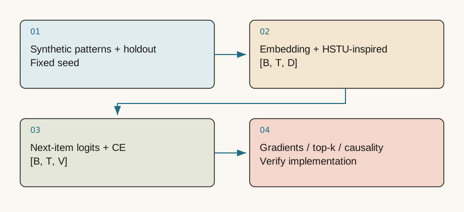
The notebook needs neither private logs nor a paid GPU. It generates controlled behavior patterns, trains a single-head model with U/Q/K/V, SiLU aggregation, gating and residuals, then produces next-item logits. Synthetic data and simplified temporal structure teach mechanics; they do not establish production impact.

IDs [B,T] become embeddings [B,T,D], the block preserves that shape, and an output head produces [B,T,V]. Every valid position can supervise next-item prediction. Padding target zero is excluded with ignore_index=0.

One backward pass is not learning evidence

Fix the seed and train deterministic sequences while plotting loss. Inspect gradient norms and compare top-k before and after training. Then test retained sequences with different starts and report actual metrics. Success on an easy synthetic rule only establishes learning within that controlled task.

# Uses model / inputs / targets defined in the complete notebook.
logits = model(inputs)
loss = torch.nn.functional.cross_entropy(
    logits.flatten(0,1), targets.flatten(), ignore_index=0)
optimizer.zero_grad(set_to_none=True)
loss.backward()
optimizer.step()

This is a training-step fragment. The notebook supplies model definitions, data, optimizer, loop, plots and assertions.

Three essential correctness checks

Changing a future token must not alter earlier outputs: test causality. Replacing padding embeddings with nonzero random values must not affect legal outputs through masked padding. Exclude reserved ID zero before top-k evaluation.

Separate falling training loss from improving validation. A training-set-only result is an implementation sanity check, not generalization. Even the notebook's held-out synthetic patterns are not a real-world independent test set.

Check your understanding

Question: Loss is low but recommendations always return ID zero. What do you inspect first?

Answer

Check padding supervision, valid targets, candidate filtering and indexing of the final valid position. You may be reading a trailing padding position instead of the sequence's real endpoint.

Actual output from this run

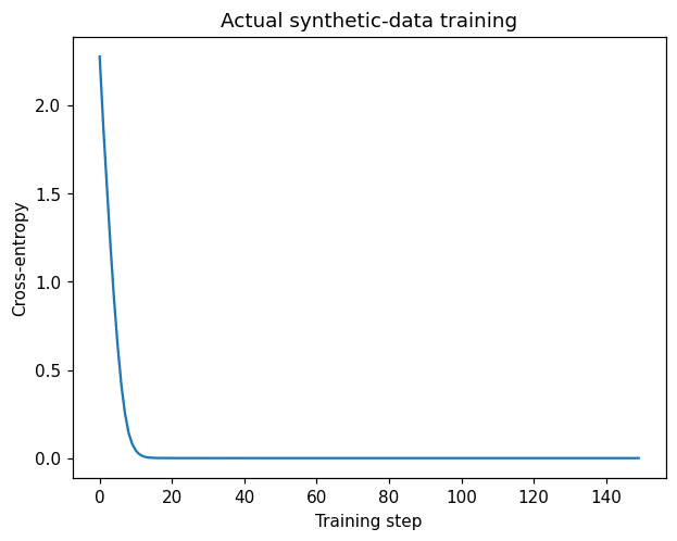
Actual training curve for the 3,538-parameter teaching model. Synthetic convergence does not establish industrial recommendation quality.

Primary sources and further reading

• Official generative-recommenders implementation
• PyTorch cross-entropy

Sources checked on 2026-09-10. Teaching examples are not production benchmarks; confirm APIs and model support against the linked version.

Actual output appears after running.